Indexing (Part 3) and Views
CSE-4/562 Spring 2019
February 22, 2019
Textbook: Papers and Ch. 8.1-8.2
Log-Structured Merge Trees
Some filesystems (HDFS, S3, SSDs) don't like updates
You don't update data, you rewrite the entire file (or a large fragment of it).
Idea 1: Buffer updates, periodically write out new blocks to a "log".
- Not organized! Slooooow access
- Grows eternally! Old values get duplicated
Idea 2: Keep data on disk sorted. Buffer updates. Periodically merge-sort buffer into the data.
- $O(N)$ IOs to merge-sort
- "Write amplification" (each record gets read/written on all buffer merges).
Idea 3: Keep data on disk sorted, and in multiple "levels". Buffer updates.
- When buffer full, write to disk as Level 1.
- If Level 1 exists, merge buffer into Level 1 to create Level 2.
- If old Level 2 exists, merge new and old to create Level 3.
- etc...
Key observation: Level $i$ is $2^{i-1}$ times the size of the buffer (the size of the level doubles with each merge).
Result: Each record copied at most $\log(N)$ times.
Other design choices
- Fanout
- Instead of doubling the size of each level, have each level grow by a factor of $K$. Level $i$ is merged into level $i+1$ when its size grows above $K^{i-1}$.
- "Tiered" (instead of "Leveled")
- Store each level as $K$ sorted runs instead of proactively merging them. Merge the runs together when escalating them to the next level.
Other design choices
- Fence Pointers
- Separate each sorted run into blocks, and store the start/end keys for each block (makes it easier to evaluate selection predicates)
- Bloom Filters
- Some data structures can be used to quickly answer lookups.
References
- "The log-structured merge-tree (LSM-tree)" by O'Neil et. al.
- The original LSM tree paper
- "bLSM: a general purpose log structured merge tree" by Sears et. al.
- LSM Trees with background compaction. Also a clear summary of LSM trees
- Monkey: Optimal Navigable Key-Value Store
- A comprehensive overview of the LSM Tree design space.
CDF-Based Indexing
"The Case for Learned Index Structures"
by Kraska, Beutel, Chi, Dean, Polyzotis
Cumulative Distribution Function (CDF)
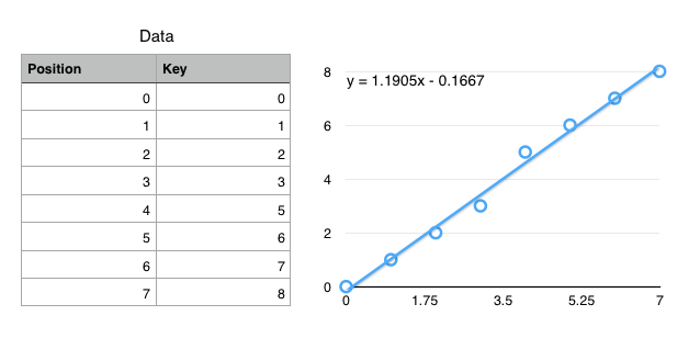
$f(key) \mapsto position$
(not exactly true, but close enough for today)
Using CDFs to find records
- Ideal: $f(k) = position$
- $f$ encodes the exact location of a record
- Ok: $f(k) \approx position$
$\left|f(k) - position\right| < \epsilon$ - $f$ gets you to within $\epsilon$ of the key
- Only need local search on one (or so) leaf pages.
Simplified Use Case: Static data with "infinite" prep time.
How to define $f$?
- Linear ($f(k) = a\cdot k + b$)
- Polynomial ($f(k) = a\cdot k + b \cdot k^2 + \ldots$)
- Neural Network ($f(k) = $
 )
)
We have infinite prep time, so fit a (tiny) neural network to the CDF.
Neural Networks
- Extremely Generalized Regression
- Essentially a really really really complex, fittable function with a lot of parameters.
- Captures Nonlinearities
- Most regressions can't handle discontinuous functions, which many key spaces have.
- No Branching
ifstatements are really expensive on modern processors.- (Compare to B+Trees with $\log_2 N$ if statements)
Summary
- Tree Indexes
- $O(\log N)$ access, supports range queries, easy size changes.
- Hash Indexes
- $O(1)$ access, doesn't change size efficiently, only equality tests.
- LSM Trees
- $O(K\log(\frac{N}{B}))$ access. Good for update-unfriendly filesystems.
- CDF Indexes
- $O(1)$ access, supports range queries, static data only.
$\sigma_C(R)$ and $(\ldots \bowtie_C R)$
Original Query: $\pi_A\left(\sigma_{B = 1 \wedge C < 3}(R)\right)$
Possible Implementations:
- $\pi_A\left(\sigma_{B = 1 \wedge C < 3}(R)\right)$
- Always works... but slow
- $\pi_A\left(\sigma_{\wedge B = 1}( IndexScan(R,\;C < 3) ) \right)$
- Requires a non-hash index on $C$
- $\pi_A\left(\sigma_{\wedge C < 3}( IndexScan(R,\;B=1) ) \right)$
- Requires a any index on $B$
- $\pi_A\left( IndexScan(R,\;B = 1, C < 3) \right)$
- Requires any index on $(B, C)$
Lexical Sort (Non-Hash Only)
Sort data on $(A, B, C, \ldots)$
First sort on $A$, $B$ is a tiebreaker for $A$,
$C$ is a tiebreaker for $B$, etc...
- All of the $A$ values are adjacent.
- Supports $\sigma_{A = a}$ or $\sigma_{A \geq b}$
- For a specific $A$, all of the $B$ values are adjacent
- Supports $\sigma_{A = a \wedge B = b}$ or $\sigma_{A = a \wedge B \geq b}$
- For a specific $(A,B)$, all of the $C$ values are adjacent
- Supports $\sigma_{A = a \wedge B = b \wedge C = c}$ or $\sigma_{A = a \wedge B = b \wedge C \geq c}$
- ...
For a query $\sigma_{c_1 \wedge \ldots \wedge c_N}(R)$
- For every $c_i \equiv (A = a)$: Do you have any index on $A$?
- For every $c_i \in \{\; (A \geq a), (A > a), (A \leq a), (A < a)\;\}$: Do you have a tree index on $A$?
- For every $c_i, c_j$, do you have an appropriate index?
- etc...
- A simple table scan is also an option
Which one do we pick?
(You need to know the cost of each plan)
These are called "Access Paths"
Strategies for Implementing $(\ldots \bowtie_{c} S)$
- Sort/Merge Join
- Sort all of the data upfront, then scan over both sides.
- In-Memory Index Join (1-pass Hash; Hash Join)
- Build an in-memory index on one table, scan the other.
- Partition Join (2-pass Hash; External Hash Join)
- Partition both sides so that tuples don't join across partitions.
- Index Nested Loop Join
- Use an existing index instead of building one.
Index Nested Loop Join
To compute $R \bowtie_{S.B > R.A} S$ with an index on $S.B$- Read one row of $R$
- Get the value of $a = R.A$
- Start index scan on $S.B > a$
- Return all rows from the index scan
- Read the next row of $R$ and repeat
Index Nested Loop Join
To compute $R \bowtie_{S.B\;[\theta]\;R.A} S$ with an index on $S.B$- Read one row of $R$
- Get the value of $a = R.A$
- Start index scan on $S.B\;[\theta]\;a$
- Return all rows from the index scan
- Read the next row of $R$ and repeat
Views
      SELECT partkey
      FROM lineitem l, orders o
      WHERE l.orderkey = o.orderkey
      AND o.orderdate >= DATE(NOW() - '1 Month')
      ORDER BY shipdate DESC LIMIT 10;
      SELECT suppkey, COUNT(*)
      FROM lineitem l, orders o
      WHERE l.orderkey = o.orderkey
      AND o.orderdate >= DATE(NOW() - '1 Month')
      GROUP BY suppkey;
      SELECT partkey, COUNT(*)
      FROM lineitem l, orders o
      WHERE l.orderkey = o.orderkey
      AND o.orderdate > DATE(NOW() - '1 Month')
      GROUP BY partkey;
All of these views share the same business logic!
Started as a convenience
      CREATE VIEW salesSinceLastMonth AS
        SELECT l.*
        FROM lineitem l, orders o
        WHERE l.orderkey = o.orderkey
        AND o.orderdate > DATE(NOW() - '1 Month')
      SELECT partkey FROM salesSinceLastMonth
      ORDER BY shipdate DESC LIMIT 10;
      SELECT suppkey, COUNT(*)
      FROM salesSinceLastMonth
      GROUP BY suppkey;
      SELECT partkey, COUNT(*)
      FROM salesSinceLastMonth
      GROUP BY partkey;
But also useful for performance
      CREATE MATERIALIZED VIEW salesSinceLastMonth AS
        SELECT l.*
        FROM lineitem l, orders o
        WHERE l.orderkey = o.orderkey
        AND o.orderdate > DATE(NOW() - '1 Month')
Materializing the view, or pre-computing and saving the view lets us answer all of the queries on the view faster!
What if the query doesn't use the view?
      SELECT l.partkey
      FROM lineitem l, orders o
      WHERE l.orderkey = o.orderkey
      AND o.orderdate > DATE(’2015-03-31’)
      ORDER BY l.shipdate DESC
      LIMIT 10;
Can we detect that a query could be answered with a view?
(sometimes)
| View Query | User Query | |
|---|---|---|
SELECT $L_v$FROM $R_v$WHERE $C_v$
|
SELECT $L_q$FROM $R_q$WHERE $C_q$
|
When are we allowed to rewrite this table?
| View Query | User Query | |
|---|---|---|
SELECT $L_v$FROM $R_v$WHERE $C_v$
|
SELECT $L_q$FROM $R_q$WHERE $C_q$
|
- $R_V \subseteq R_Q$
- All relations in the view are part of the query join
- $C_Q = C_V \wedge C'$
- The view condition is 'weaker' than the query condition
- $attrs(C') \cap attrs(R_V) \subseteq L_V$ $L_Q \cap attrs(R_V) \subseteq L_V$
- The view doesn't project away needed attributes
| View Query | User Query | |
|---|---|---|
SELECT $L_v$FROM $R_v$WHERE $C_v$
|
SELECT $L_q$FROM $R_q$WHERE $C_q$
|
SELECT $L_Q$FROM $(R_Q - R_V)$, viewWHERE $C_Q$
Summary
- For each relation, identify candidate indexes
- For each join, identify candidate indexes
- Identify candidate views
- Identify available join, aggregate, sort algorithms
Enumerate all possible plans
... then how do you pick? (more next class)